Working with Cactus horizons

In this notebook, we learn how to work with horizon data.

(This notebook is meant to be converted in Sphinx documentation and not used directly.)

import matplotlib.pyplot as plt
import numpy as np
from kuibit.simdir import SimDir

%matplotlib inline

The best way to access horizon data is from SimDir:

hor = SimDir("../../tests/horizons").horizons

print(hor)

Horizons found:
3 horizons from QuasiLocalMeasures
2 horizons from AHFinderDirect

As we see, kuibit found some horizons. kuibit looks for data from QuasiLocalMeasures and AHFinderDirect. These two thorns use different indexing systems, and, at the moment, you must provide both to uniquely indentify an horizon. If you need information from only one of the two (e.g., you want to plot the apparent horizon), you can also use the functions get_apparent_horizon and get_qlm_horizon.

h1 = hor[(0, 1)]
print(h1)

Formation time: 0.0000
Shape available
Final Mass = 5.538e-01
Final Angular Momentum = -3.598e-07
Final Dimensionless Spin = -1.173e-06

You can find the available indices using suitable attributes:

print(hor.available_qlm_horizons)
print(hor.available_apparent_horizons)

[0, 1, 2]
[1, 2]

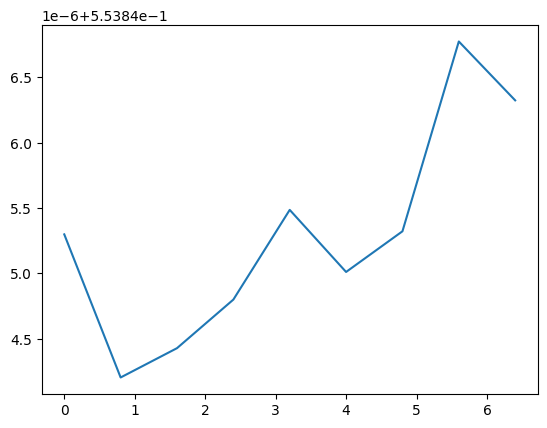
Once an horizon is fixed, you can access all the properties from QuasiLocalMeasures and from AHFinderDirect as attributes. These are all TimeSeries. For example, the mass as computed by QuasiLocalMeasures:

plt.plot(h1.mass)

[<matplotlib.lines.Line2D at 0x7f7f3abe5e10>]

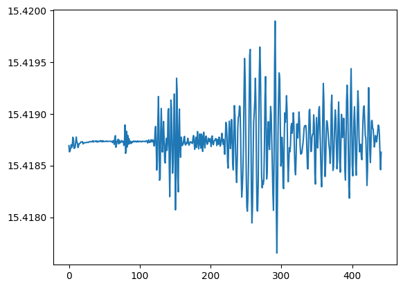
For quantities from AHFinderDirect you have to use the ah namespace:

plt.plot(h1.ah.area)

[<matplotlib.lines.Line2D at 0x7f7f3ab71690>]

kuibit can also work with shape data. AHFinderDirect uses multiple patches, we can plot an example in 3D:

from mayavi import mlab
mlab.init_notebook('png')

(px, py, pz) = h1.shape_at_iteration(0)

mlab.mesh(px[0], py[0], pz[0], representation='wireframe')

Notebook initialized with png backend.

If you plot all the patches, you will have the horizon in 3D.

mlab.clf()

for pnum in range(len(px)):
    mlab.mesh(px[pnum], py[pnum], pz[pnum], color=(0, 0, 0))

# For some reasons mlab.show() doesn't produce the picture here,
# so, there' is an additional mlab.mesh statement. This is here
# just to display the picture
mlab.orientation_axes()
mlab.mesh(px[0], py[0], pz[0], color=(0,0,0))

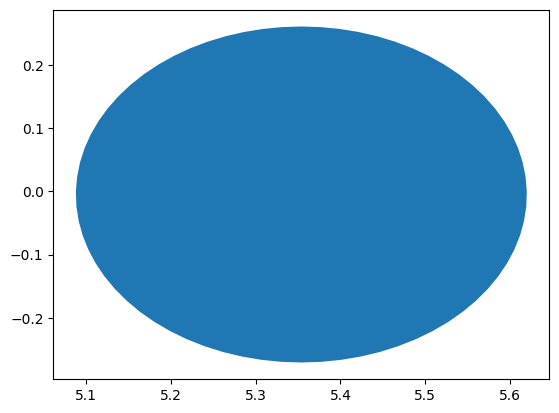
In case you want to work with a 2D slice, of the shape, you can use the method shape_outline_at_iteration and specify how to cut the shape.

Note that the the distributions of points is not uniform across the horizon and kuibit does not do any interpolation across points. Therefore, there are values of cut that will lead to a malformed horizon. It is recommended to use cuts that are along the principal directions.

cut = [None, None, 0]  # Equatorial plane (z=0)

shape = h1.shape_outline_at_iteration(0, cut)

plt.fill(*shape)

[<matplotlib.patches.Polygon at 0x7f7f1f9db890>]

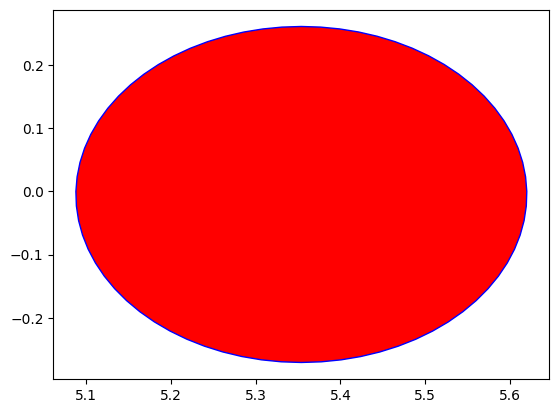
You can also use the module visualize_matplotlib to plot the horizon in 2D. If you already have the shape, you can use plot_horizon.

from kuibit import visualize_matplotlib as viz

viz.plot_horizon(shape, color='r', edgecolor='b')

[<matplotlib.patches.Polygon at 0x7f7f1e5e2590>]

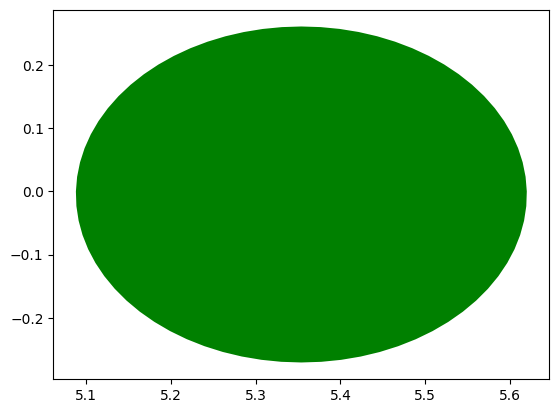
Alternatively, you can use the higher level functions plot_horizon_on_plane_at_iteration or plot_horizon_on_plane_at_time. These take directly a OneHorizon object and the desired iteration/time.

viz.plot_horizon_on_plane_at_time(h1, time=0, plane="xy", color='g')

[<matplotlib.patches.Polygon at 0x7f7f1e45bdd0>]