Working with grid data

In this notebook, we show some of the most useful features of the grid_data module.

There are three important objects in grid_data: - UniformGrid represents Cartesian grids, - UniformGridData represents data on UniformGrid, - HierarchicalGridData represents data on multiple grids with different spacings (a mesh-refined grid).

In most cases you will not define these objects directly, but it is important to know how they work. To learn how to read the simulation data, see working with grid funcitons.

(This notebook is meant to be converted in Sphinx documentation and not used directly.)

import matplotlib.pyplot as plt
import numpy as np
from kuibit import grid_data as gd
from kuibit import grid_data_utils as gdu
from kuibit import series

%matplotlib inline

UniformGrid

To generate data, we start from preparing a grid. kuibit follows the conventions in Carpet and identifies a grid with (1) the number of points along each direction, (2) the coordinate of left bottom cell, (3) the spacing or the coordinate of the top right cell. In addition, UniformGrid can contain additional information, like the number of refinement level, or the time. These grids are always cell-centered.

Let us create a 2D grid:

grid = gd.UniformGrid([201, 201], # Number of points
                      x0=[-100, -100], # origin
                      x1=[100, 100] # other corner
                      )

UniformGrid are meant to be immutable objects, and indeed there is not much that we can do with them. If we print them, we will find some interesting information.

print(grid)

Shape            = [201 201]
Num ghost zones  = [0 0]
Ref. level       = -1
Component        = -1
x0               = [-100. -100.]
x0/dx            = [-100. -100.]
x1               = [100. 100.]
x1/dx            = [100. 100.]
Volume           = 40401.0
dx               = [1. 1.]
Time             = None
Iteration        = None

We can obtain this (and other information) directly from grid, for example.

print(f"Unit volume {grid.dv}, number of dimensions {grid.num_dimensions}")

Unit volume 1.0, number of dimensions 2

UniformGrid objects can be indexed and support the in operator, which are quite convinent.

print(f"The coordinate cooresponding to the index 1, 2 is {grid[1,2]}")
print(f"Is [-140, 50] in the grid?: {[-140, 50] in grid}")

The coordinate cooresponding to the index 1, 2 is [-99. -98.]
Is [-140, 50] in the grid?: False

Finally, one can get explicitly the coordinates with the coordinates method. This can return arrays with the coordinates along each direction (default), or can return the coordinates as a numpy meshgrid (if as_meshgrid=True), or can return a list of arrays with the same shape of the grid and the values of the coordinates (if as_same_shape=True). Let’s see one example.

print(grid.coordinates()[0])

[-100.  -99.  -98.  -97.  -96.  -95.  -94.  -93.  -92.  -91.  -90.  -89.
  -88.  -87.  -86.  -85.  -84.  -83.  -82.  -81.  -80.  -79.  -78.  -77.
  -76.  -75.  -74.  -73.  -72.  -71.  -70.  -69.  -68.  -67.  -66.  -65.
  -64.  -63.  -62.  -61.  -60.  -59.  -58.  -57.  -56.  -55.  -54.  -53.
  -52.  -51.  -50.  -49.  -48.  -47.  -46.  -45.  -44.  -43.  -42.  -41.
  -40.  -39.  -38.  -37.  -36.  -35.  -34.  -33.  -32.  -31.  -30.  -29.
  -28.  -27.  -26.  -25.  -24.  -23.  -22.  -21.  -20.  -19.  -18.  -17.
  -16.  -15.  -14.  -13.  -12.  -11.  -10.   -9.   -8.   -7.   -6.   -5.
   -4.   -3.   -2.   -1.    0.    1.    2.    3.    4.    5.    6.    7.
    8.    9.   10.   11.   12.   13.   14.   15.   16.   17.   18.   19.
   20.   21.   22.   23.   24.   25.   26.   27.   28.   29.   30.   31.
   32.   33.   34.   35.   36.   37.   38.   39.   40.   41.   42.   43.
   44.   45.   46.   47.   48.   49.   50.   51.   52.   53.   54.   55.
   56.   57.   58.   59.   60.   61.   62.   63.   64.   65.   66.   67.
   68.   69.   70.   71.   72.   73.   74.   75.   76.   77.   78.   79.
   80.   81.   82.   83.   84.   85.   86.   87.   88.   89.   90.   91.
   92.   93.   94.   95.   96.   97.   98.   99.  100.]

UniformGridData

UniformGridData are much more interesting. UniformGridData packages a UniformGrid and some data in the same object and provides many useful functionalities.

Let us create some fake data to explore the capabilities. A simple way to generate a UniformGridData from a function is with sample_function.

grid_data = gdu.sample_function(lambda x, y: x * y,
                          [101, 201], # shape
                          [0, 0], # origin
                          [10, 10] # other corner
                          )

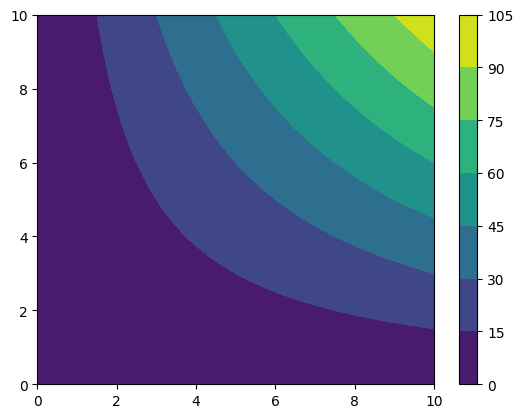
We can visualize this data with matplotlib contourf. To do this, we need the coordinates as meshgrid, and we need the actual data. To get the first, we use the coordinates_meshgrid method, for the second, we access directly the data with the data attribute. This is stored as a numpy array. Often, we want to plot these objects. Using data directly would lead to transposing the actual physical quantity, because data is a matrix stored by rows, so, the first index does not label the x coordiante, but the y. We provide the aliaxs data_xyz, which is the the tranposed of data. This is ready to be plotted.

⚠️ In this tutorial, we plot the various quantities directly. This is to understand to access the data and what is the fundamental structure of these objects. However, kuibit comes with plottings methods too. The visualize_matplotlib module contains multiple functions to make 2D plots. We touch upon this at the end of this tutorial.

cf = plt.contourf(*grid_data.coordinates_meshgrid(), # The star is to unpack the list
                  grid_data.data_xyz)
plt.colorbar(cf)

<matplotlib.colorbar.Colorbar at 0x7f3094038b00>

UniformGridData support all the mathematical operations we may want, for instance.

funky_data = np.sqrt(grid_data) + grid_data**2 * np.tanh(grid_data)
cf = plt.contourf(*funky_data.coordinates_meshgrid(), funky_data.data_xyz)
plt.colorbar(cf)

<matplotlib.colorbar.Colorbar at 0x7f3093fff0e0>

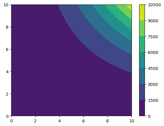
We can find the absolute maximum and where the coordinate where the absolute maximum is reached (the argument absolute=False would be required if we did not want the absolute).

print(f"The absolute maximum is {funky_data.abs_max()}")
print(f"The absolute maximum occurs at {funky_data.coordinates_at_maximum()}")

The absolute maximum is 10010.0
The absolute maximum occurs at [10. 10.]

UniformGridData can be interpolated with splines to evalute data everywhere, even where there was no data. With this, we can make UniformGridData callable objects:

print(f"The value of funky_data at (2, 3) is {funky_data((2,3)):.3f}")

The value of funky_data at (2, 3) is 38.449

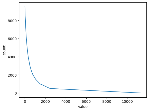
UniformGridData have built-in a collection of useful functions, for example:

print(f"The mean of funky_data is {funky_data.mean():.3f}")
print(f"The integral of funky_data is {funky_data.integral():.3f}")
print(f"The norm2 of funky_data is {funky_data.norm2():.3f}")

bins, hist = funky_data.histogram(num_bins=20)
plt.ylabel("count")
plt.xlabel("value")
plt.plot(bins, hist[:-1])

The mean of funky_data is 1123.865
The integral of funky_data is 114077.947
The norm2 of funky_data is 20417.836

[<matplotlib.lines.Line2D at 0x7f3094017a40>]

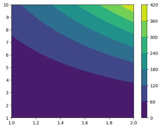
It is not possible to combine directly two UniformGridData with different associated grids, but it is always possible to resample the objects so that they have a common grid.

Pay attention: resampling operations can be very expensive with large grids or high dimensions!

new_grid = gd.UniformGrid([201, 301], x0=[1, 1], x1=[2, 10])
resampled_funky = funky_data.resampled(new_grid)
cf = plt.contourf(*resampled_funky.coordinates_meshgrid(), resampled_funky.data_xyz)
plt.colorbar(cf)

<matplotlib.colorbar.Colorbar at 0x7f3093db6780>

Being able to resample UniformGridData means that even if it is not possible to directly combine objects with different grids, you can always resample them to a common grid, and then perform the operation.

Often, it is useful to save a UniformGridData to disk. A common example is to resampled 3D grid data on a cluster and move the much smaller saved file to a local computer or laptop.

This can be achieved with the save method and the load_UniformGridData function.

resampled_funky.save("/tmp/funky.npz")

from kuibit.grid_data_utils import load_UniformGridData

loaded_data = load_UniformGridData("/tmp/funky.npz")

The fastest format to save data in is npz, but this is not always portable. The save method accepts many other formats, like txt, dat, and also compressed ones (e.g., txt.gz).

HierarchicalGridData

Now that we have some familiarity with UniformGridData, we can move to the most important object, HierarchicalGridData. The relevance of this class is due to the fact that simulation data is represented with HierarchicalGridData objects.

A HierarchicalGridData is a collection of UniformGridData, or (or more) for each refinement level.

Let us prepare some fake data.

# 3 refinement levels
data = []
for ref_level in range(3):
    resolution = (1 + ref_level) * 20 + 1
    data.append(gdu.sample_function(lambda x, y: x*y + 5,
                                   [resolution, resolution],
                                   [-10, -10],
                                   [10, 10],
                                   ref_level=ref_level
                                   ))
hg = gd.HierarchicalGridData(data)
print(hg)

Available refinement levels (components):
0 (1)
1 (1)
2 (1)
Spacing at coarsest level (0): [1. 1.]
Spacing at finest level (2): [0.33333333 0.33333333]

“Components” are essentially patches of grid. In some cases, components are a result of running the code on multiple processes. In this case, kuibit will try to merge them in a single grid. In other instances, when there are multiple centers of refinement, the components are real. Here, kuibit will do nothing and will keep all the components around.

To access a specific refinement level, we can use the backet operator. This will return a list of all the components at that level. Often, there will be only one element because kuibit successfully merged the various patches. In this case, one can use the get_level method to get directly the data on that level.

level2 = hg.get_level(2)

type(level2)

kuibit.grid_data.UniformGridData

As we see, this is just a UniformGridData, so everything we can operate on single levels exactly in the same way we work on UniformGridData. If the HierarchicalGridData has multiple disconnected components, hg[2] will instead return a list of UniformGridData.

HierarchicalGridData fully support mathematical operations. (Binary operations are performed only if the two objects have the same grids and components.)

more_funk = (abs(hg) + 2).log() # For some reasons np.log(hg) doesn't work...

# We can also call the HierarchicalGridData
print(f"more_funk of (2, 3) is {more_funk((2,3)):.3f}")

more_funk of (2, 3) is 2.565

We cannot plot directly this object, because it is a complicated object. To plot it, we have to merge the refinement levels to a single UniformGridData. We can do this with refinement_levels_merged().

Note that refinement_levels_merged is a very expensive operation and that it is provided only for small datasets or for one-dimensional data.

merged = more_funk.refinement_levels_merged(resample=True)
cf = plt.contourf(*merged.coordinates_meshgrid(), merged.data_xyz)
plt.colorbar(cf)

<matplotlib.colorbar.Colorbar at 0x7f3093e5f3e0>

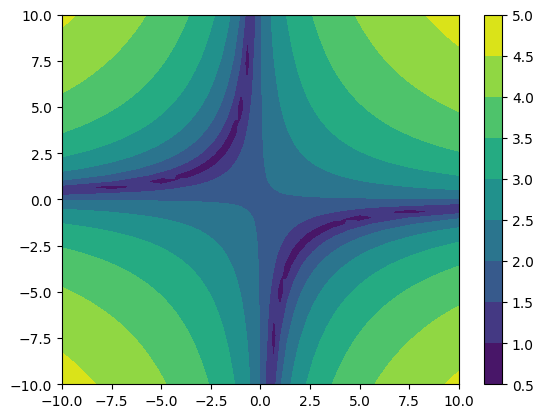
As you noticed, we enabled the resample option. With this option the coarser refinement levels are interpolated to the new finer grid using multilinear interpolation.

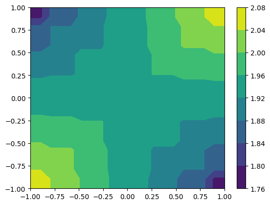
When working with large grids, many refinement levels, and/or 3D data, merging the various refinement levels can be a very expensive operation. However, often we don’t need the entire grid, but we want to look at a portion. HierachicalGridData objects have a method to merge the refinement levels on a specified grid.

small_funk = more_funk.to_UniformGridData([20, 20], x0=[-1, -1], x1=[1, 1], resample=False)
cf = plt.contourf(*small_funk.coordinates_meshgrid(), small_funk.data_xyz)
plt.colorbar(cf)

<matplotlib.colorbar.Colorbar at 0x7f30940d5d60>

HierachicalGridData objects have a lot of information that is accessible as a property.

print(f"Available refinement levels: {hg.refinement_levels}")
print(f"Spacing of the coarsest: {hg.coarsest_dx}")
print(f"Spacing of the finest: {hg.finest_dx}")
print(f"Finest level: {hg.finest_level}")

Available refinement levels: [0, 1, 2]
Spacing of the coarsest: [1. 1.]
Spacing of the finest: [0.33333333 0.33333333]
Finest level: <kuibit.grid_data.UniformGridData object at 0x7f3093d8f740>

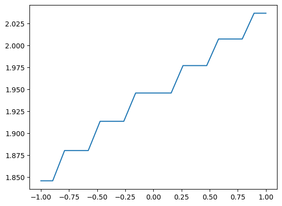
Often, we want to look at a specific cut of the data. UniformGridData can be sliced easily. Just prepare a cut array with None where you want to keep the dimension, and the coordiante of where you want to slice. For example, here we extract the line with y=0.7.

along_y = small_funk.sliced([None,0.7])
print(along_y.grid)
plt.plot(*along_y.coordinates_meshgrid(), along_y.data)

Shape            = [20]
Num ghost zones  = [0]
Ref. level       = -1
Component        = -1
x0               = [-1.]
x0/dx            = [-9.5]
x1               = [1.]
x1/dx            = [9.5]
Volume           = 2.1052631578947367
dx               = [0.10526316]
Time             = None
Iteration        = None

[<matplotlib.lines.Line2D at 0x7f3091bb7a40>]

When working with a one-dimensional array, you can consider converting it to a GridSeries with the method to_GridSeries. That is: instead of using the entire infrastructure for grid data, you can use the infrastructure for series (e.g., TimeSeries). The main advantage is that the series infrastrcture is more direct and lean. For example, you can plot directly with plt.plot().

along_y_series = along_y.to_GridSeries()
plt.plot(along_y_series)

[<matplotlib.lines.Line2D at 0x7f3093d8eb70>]

Masks

It is often useful to mask the data according to some criterion. For example, mask the atmosphere out in a GRMHD simulation. kuibit fully supports mask with an interface that is similar to the one implemented in NumPy (but some features will not work with masked data, for example interpolation).

The module kuibit.masks provides methods to apply masked functions in case the domain is restricted. For example, for the logarithm, or arcsin:

import kuibit.masks as km

arcsin_funk = km.arcsin(more_funk)

print(arcsin_funk.is_masked())

True

Alternatively, it is possible to apply masks according to the value of the data. For instance, masking all the values smaller than a given one:

print(more_funk.abs_min())

funk_masked = more_funk.masked_less(1)

print(funk_masked.abs_min())  # The minimum now reflects the mask

0.6931471805599453
1.0116009116784799

You can extract the mask and apply to another grid variable with the same structure. (This is how you would apply the atmospheric mask to other grid functions).

funk2 = more_funk ** 2

funk2_masked = funk2.mask_applied(funk_masked.mask)

print(funk2_masked.is_masked())

True

visualize_matplotlib

In this tutorial we plotted all the quantities directly accessing the data. This is a pedagogical choice: you need to know how things work to be able to take full advantage of kuibit. However, most often the methods in the module visualize_matplotlib will be enough.

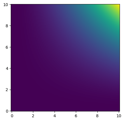
The main functions to plot 2D data are: plot_color and plot_contourf. These take all sorts of inputs, and you should read the documentation. For example, we can plot a UniformGridData (the function will behave similarly with HierarchicalGridData or NumPy arrays).

import kuibit.visualize_matplotlib as viz

viz.plot_color(funky_data)

<matplotlib.image.AxesImage at 0x7f30940d6f90>

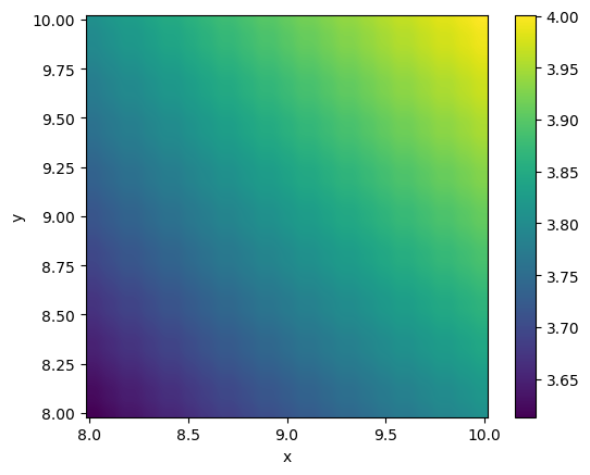
If we are only interested in a smaller region (and setting other parameters):

viz.plot_color(funky_data, x0=[8,8], x1=[10,10],
               shape=[50, 50], colorbar=True,
               logscale=True, xlabel="x", ylabel="y",
               interpolation="bicubic")

<matplotlib.image.AxesImage at 0x7f3091d276b0>

The method plot_contourf works in the same way.

If the data has some symmetries (e.g., reflection or rotation), those can be undone to improve the image. To do so, use the reflection_symmetry_undo or rotation180_symmetry_undo methods.